State Minimum Wage Increases and Low-Wage Employment

Key Metrics

Sample

50 states, quarterly 2015–2022 (1,260 obs) — 19 treated, 26 control, 5 excluded

Model A, β₃ (avg. effect)

−0.020 food service (p=0.22), −0.009 retail (p=0.44); only food service is significant in the ≥$0.50 subsample

Model C, β₄ (exposure gradient)

0.143 food service (p=0.43), −0.006 retail (p=0.94) — noisy and inconsistent in sign

Robustness on β₄

4/4 independent checks (placebo, permutation, event study, spec curve) flag it as confounded

Wage pass-through

13% (food service proxy, p=0.65) / 63% (retail proxy, p=0.22) of the mandated increase — neither significant

Treatment predictability

Logistic regression on pre-period growth + exposure: 87% accuracy, AUC 0.97 — highly predictable

State clustering

k-means (k=3): 2 of 3 clusters are essentially pure treated/control (χ² p<0.0001)

Inference

State-clustered SEs, wild cluster bootstrap, 10,000-rep permutation test, Monte Carlo power analysis

Engineering

32 R scripts, 369 R assertions + 61 Python tests (all passing), CI on every push

Results at a Glance

Question	Result	Interpretation
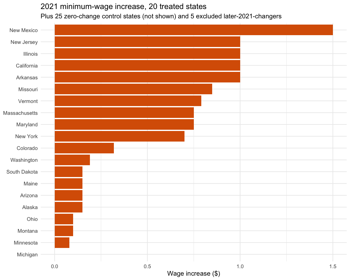
Average employment effect	Negative but not robust	Weak causal evidence
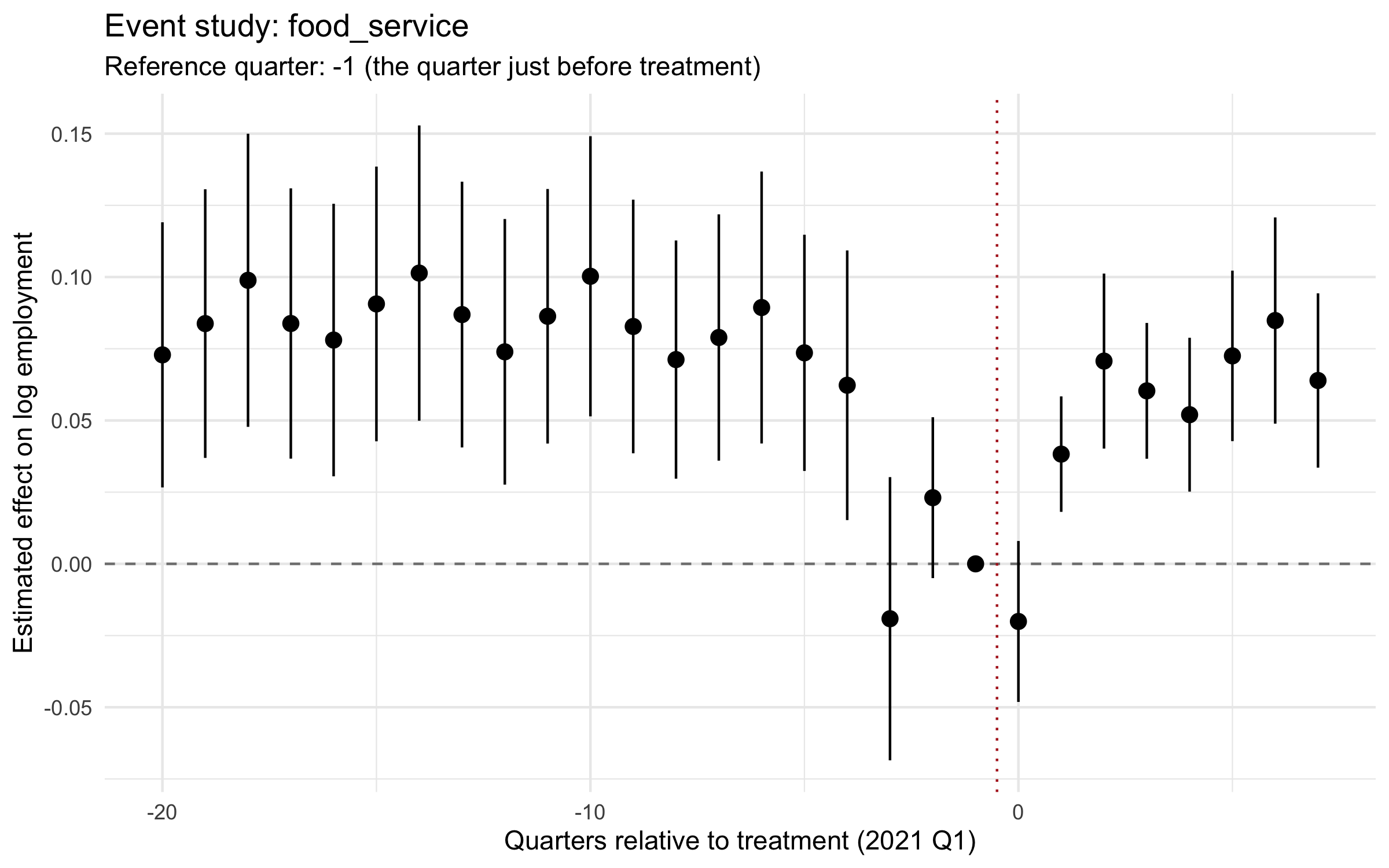
Parallel trends	Rejected for both industries (event-study joint tests)	Major identification concern
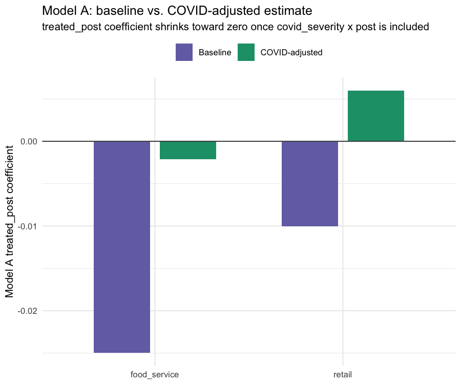
COVID sensitivity	Large change once controlled for	Confounding likely
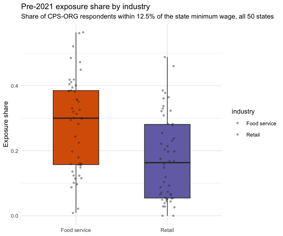
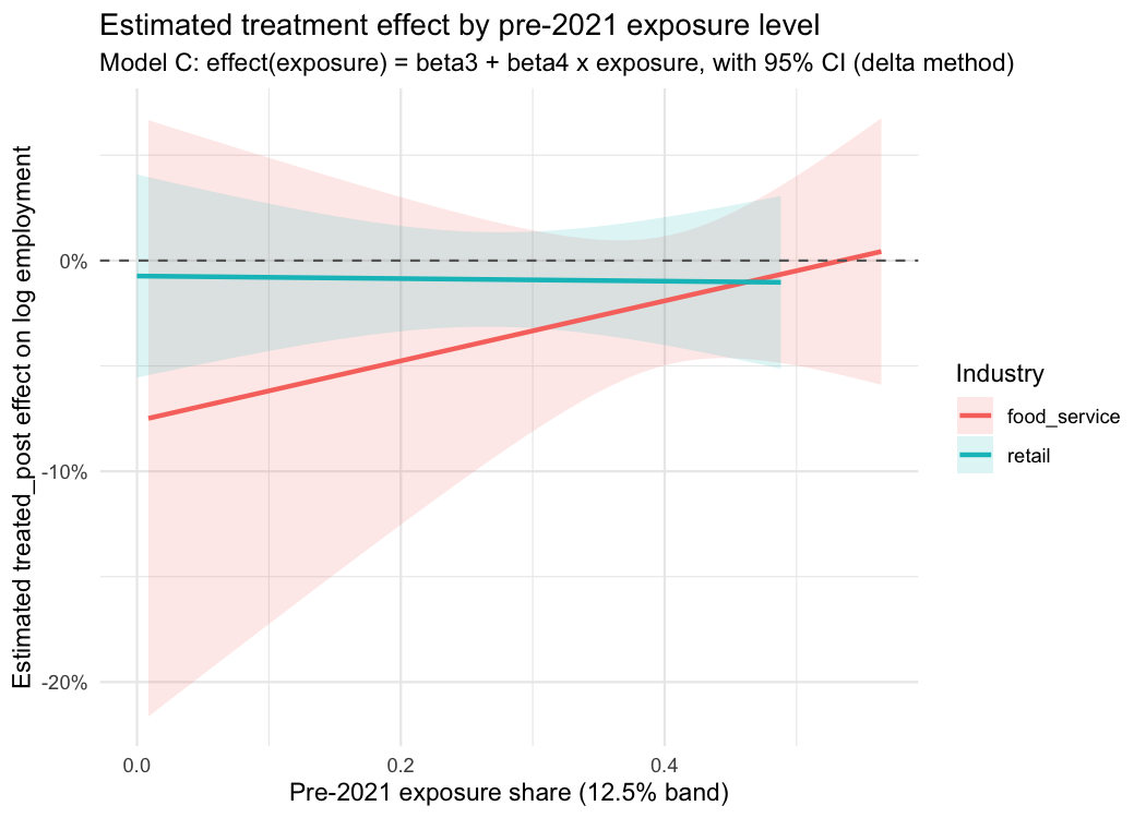
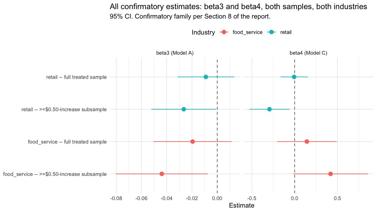
Exposure gradient (β₄)	Inconclusive and confounded	Underpowered, not "no effect"
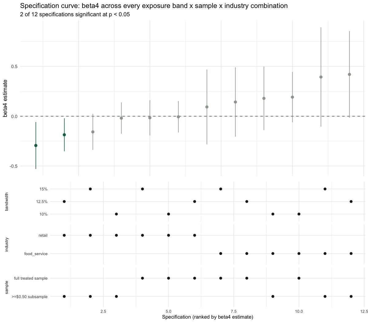
Placebo / permutation / event study / spec curve (β₄)	All 4 flag a pre-existing exposure–outcome link	Convergent evidence, not one fluke
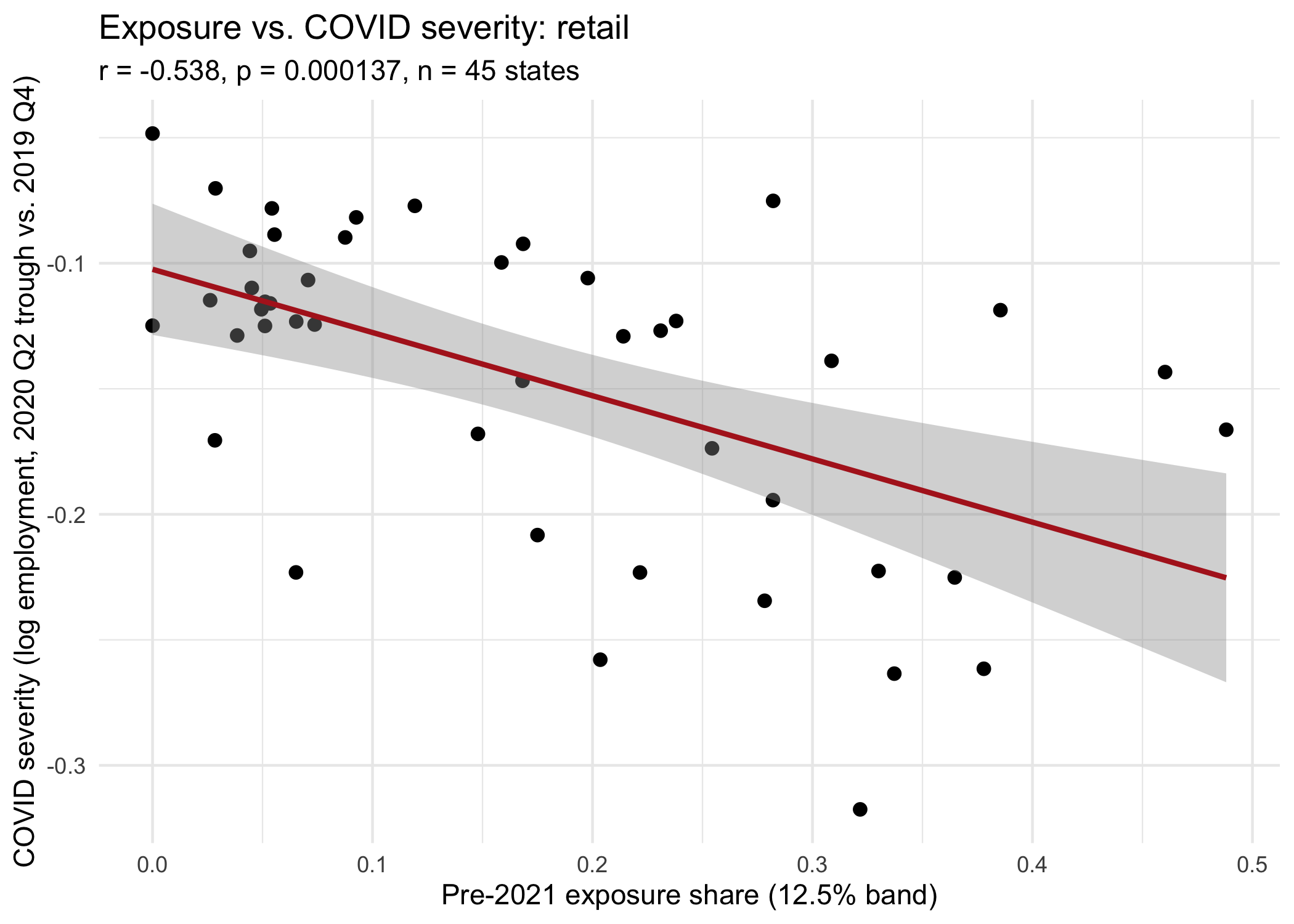
Exposure vs. COVID severity	Significant negative correlation	A candidate mechanism — but barely moves the placebo effect once controlled for
Multiple-testing correction	None of the 4 confirmatory tests survive Holm	Consistent with "not robust," now formal
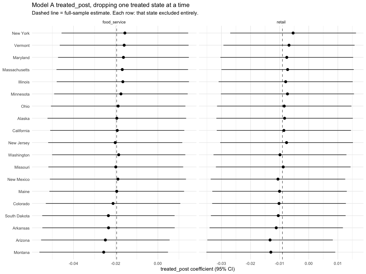
Leave-one-state-out	Estimate stable across all 19 drops	No single state drives Model A
Wage pass-through	13%/63% of the mandated increase, neither significant	Consistent with underpowered, not "no pass-through"
Is treatment predictable from pre-period data?	Yes — 87% accuracy, AUC 0.97	Another angle on non-random assignment
Do states cluster by treatment status?	Yes — 2/3 k-means clusters are nearly pure	Convergent with the predictability result

Key Figures

Map/chart of which states were treated and by how much — Which states were treated, and by how much

Event study showing pre-trends for food service — Event study: pre-trends don't hold for food service

Baseline vs COVID-adjusted estimate comparison — Baseline vs. COVID-adjusted estimate

Pre-2021 exposure distribution by industry

Marginal effects of exposure on treatment effect — Does the treatment effect scale with exposure?

Forest plot of all four confirmatory estimates — All four confirmatory estimates at a glance

Specification curve across band, sample, and industry choices — Every reasonable band × sample × industry choice, ranked

Exposure predicts COVID severity correlation — Exposure predicts COVID severity — a candidate confound mechanism

Leave-one-out sensitivity of Model A treated_post coefficient — Leave-one-state-out: no single state drives the estimate

Wage Pass-Through

A new research question, not a re-analysis of the one above: did the 2021 increases actually raise earnings in low-wage industries, and by how much relative to the dollar size of the mandate? Everything above asks whether employment fell; this asks whether the policy did the thing it was actually meant to do.

Data limitation, found by direct request: BLS/FRED don't publish state-level average hourly earnings at the detailed NAICS-722 (food service) or 44-45 (retail trade) level the employment analysis uses — every candidate series ID at that resolution 404s. The finest available breakdown is the CES supersector: "Leisure and Hospitality" (nests food service, but also accommodation and arts/entertainment/recreation) as the food-service proxy, and "Trade, Transportation, and Utilities" (nests retail, but also wholesale trade, transportation, and utilities) as the retail proxy. Both are broader than this study's employment industries — a real limitation, not a rounding error.

Grey = average mandated statutory increase · Red = estimated proxy-industry wage effect (hover for exact values)

Proxy industry	treated_post (log pts)	p	Mandated $/hr	Estimated $/hr	Pass-through
Leisure & Hospitality (food service proxy)	0.0044	0.647	$0.54	$0.07	13%
Trade, Transportation & Utilities (retail proxy)	0.0144	0.217	$0.54	$0.34	63%

Neither estimate is statistically significant, and the food-service proxy's confidence interval crosses zero on both sides — consistent with this study's broader theme that these designs are underpowered at the observed effect sizes, not evidence that pass-through is genuinely 13%/63%. The likeliest reason both estimates sit well under 100%: the supersector proxies include large numbers of workers (hotel managers, arts/entertainment/recreation staff, wholesale and utilities employees) who were never near the minimum wage to begin with, diluting any real effect on the low-wage workers actually targeted. See R/29_wage_passthrough.R for the full specification (it reuses Model A's fixed-effects DiD unchanged, just on a different outcome).

Treatment Assignment: Predictability & Clustering

Exploratory analyses investigating systematic differences in pre-treatment economic structure between treated and comparison states, using techniques not used elsewhere in this project (chi-square test of independence, logistic regression as a classifier, k-means, PCA).

Check	Result	Method
Treatment status vs. Census region	Not independent (χ²=8.0, p=0.046)	Chi-square test
Treatment status from pre-period growth + exposure	87% accuracy, AUC 0.97	Logistic regression, n=45
States cluster by pre-period profile	2/3 clusters nearly pure treated/control (χ²=28.0, p<0.0001)	Hand-rolled k-means + PCA

Predicted probability of treatment by state, colored by actual treatment status — Predicted P(treated) by state — logistic regression, 87% accuracy

PCA scatter plot of k-means clusters colored by cluster, shaped by treatment status — k-means clusters (color) vs. treatment status (shape) on the first 2 principal components

This does not, by itself, invalidate the causal design. DiD does not require random treatment assignment — a highly predictable treatment is entirely compatible with valid causal identification, provided the relevant conditional parallel-trends assumption holds. What these results actually motivate is taking the event study's direct test of that assumption seriously: for both industries, event-study pre-trends are rejected (see Limitations above), and that — not the predictability or clustering results here — is this study's real identification problem. Exploratory, not a fourth confirmatory test: no cluster-based hypothesis was pre-registered. 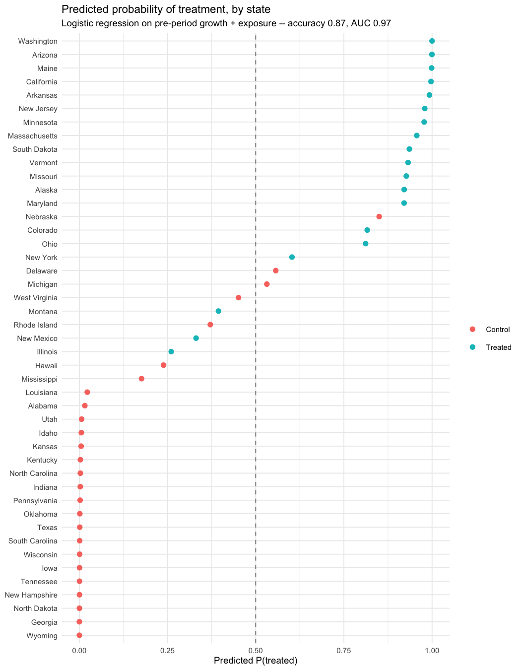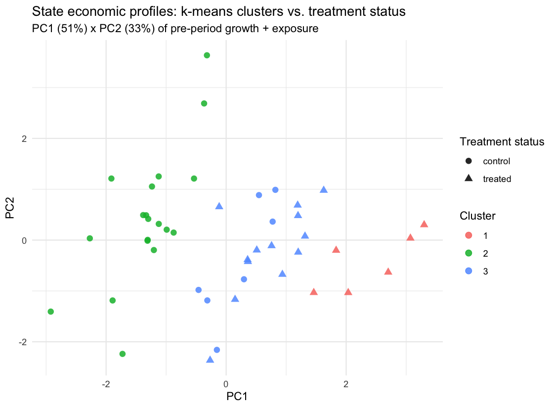See R/30_treatment_predictability.R and R/31_state_clustering.R.

Machine Learning & Neural Network Extension

A predictive-accuracy comparison, kept separate from the causal claims above: how well can flexible ML methods predict quarterly employment growth for a state they never saw during training, versus a plain linear specification? States — not rows — are held out, since a row-level split would leak within-state structure the causal models' clustered standard errors already treat as non-independent.

R implementation

Extends the study's own pipeline (R/27_ml_prediction.R, R/28_neural_network.R):

Linear baseline (no fixed effects, so it can generalize to an unseen state)
Hand-rolled bagged-trees ensemble — bootstrap-aggregated rpart trees, one fixed random feature subset per tree
Real random forest (randomForest package) — re-samples the feature subset at every split, not once per tree
Real gradient boosting (gbm package) — sequential trees fit to residuals, with the number of trees chosen by 5-fold cross-validation
Single-hidden-layer neural network (nnet), with train-only standardization

Python implementation

An independent replication in a separate ecosystem (python/), reading the same exported panel:

OLS via closed-form normal equations (numpy)
A regression tree built from scratch, with a bagging ensemble, a true random forest, and gradient boosting (sequential residual fitting) on top of it
PyTorch feedforward neural network
Pytest coverage checks, linting, type checks, a package-build check, and a separate virtual environment

Held-out R² by state (R implementation) · hover a bar for RMSE too

Model	RMSE	R²
Linear baseline	0.0699	0.394
Bagged trees	0.0667	0.448
Random forest	0.0643	0.487
Gradient boosting	0.0536	0.644
Neural network	0.0582	0.580

Gradient boosting is the strongest predictor of the five — a sensible result, not a foregone one, since boosting's sequential residual-fitting strategy is genuinely different from bagging and random forests' independent-trees-then-average strategy. This is a methods comparison, not a substitute for Model A/C's identification strategy — a model that predicts employment well isn't thereby estimating the policy's causal effect on it. See python/README.md for implementation notes.

Python Causal ML and Results API

The Python package includes state-grouped cross-validation, grid search, cluster bootstrap intervals and permutation importance. Its causal extension uses cross-fitted double ML and an exposure-specific linear R-learner.

These exploratory estimates use employment growth and region controls, rather than Model A/C's log employment and state/quarter fixed effects. They do not reproduce the same estimand or repair failed parallel trends. DML standard errors cluster by state with a finite-cluster correction. Its normal-approximation intervals assume independent states and adequate nuisance fits; they do not resolve confounding or cross-state shocks.

A read-only FastAPI service serves precomputed comparison, tuning and causal-ML CSVs. It does not train models or accept prediction requests. Missing result files return HTTP 404. This static website's two charts display saved R results; they are not connected to a deployed API.

See the Python documentation for setup and endpoints.

Limitations

Parallel trends violated for both industries in the event study; the separate two-sample test rejects for food service only.
COVID-era differential recovery confounds the treatment window — a real share of the baseline estimate, not the policy.
Both β₃ and β₄ are underpowered at the observed effect sizes, not just assumed underpowered.
β₄ is also confounded, not just underpowered — 4 independent checks find high/low-exposure states already differed before 2021.
The ≥$0.50 subsample and the legislated-only subsample are the exact same 10 states — the two cuts can't be disentangled in this data.
Small cluster count (19 treated, 45 total) — addressed via clustered SEs and a wild bootstrap, but always some caution.
Wage pass-through uses broader supersector proxies, not the exact food-service/retail industries — BLS/FRED don't publish earnings at that resolution by state.
Results are DiD estimates under this specification, not definitive causal effects.

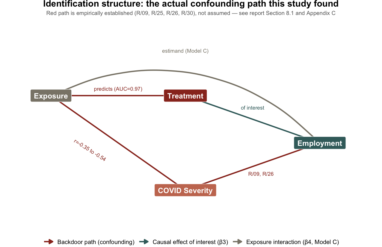
Identification structure: not a generic textbook DAG — the red path below is this study's own confounding structure, established empirically (exposure predicts treatment status: R/30; exposure correlates with COVID severity: R/25-R/26), not assumed.

Identification diagram showing the confounding backdoor path from exposure through treatment and COVID severity to employment

Data Sources

FRED (public API)

State-quarter employment, GDP, population, 2015–2022

U.S. DOL

Minimum wage history — treatment classification

QCEW Open Data API

Fallback employment (2 states); validation check

CPS-ORG via IPUMS-CPS

Exposure construction (2019–2020 earnings only)

FRED CES avg. hourly earnings (supersector)

Wage pass-through analysis (R/29)

How to Reproduce

Rscript -e 'renv::restore()'   # pinned package versions (renv.lock, R 4.5.1)
make all                       # R/01-R/32, tests, figures, report end to end
make test                      # just the R test suite
make report-pdf                # PDF export (headless Chrome, no LaTeX needed)

make python-setup              # one-time: creates python/.venv, installs the minwage package
make python-test                # Python ML/NN test suite (python/)

make all needs IPUMS_API_KEY in .env for R/03, and takes several minutes. Full details and repo layout are in the README.